In Chapter 2 of Bayesian Methods for Hackers, there's an example of Bayesian analysis of an A/B test using simulated data. I decided to play around with this analysis method with real A/B landing page test data from one of my clients.

This method uses PyMC to estimate the real conversion rate for each page and Matplotlib to visually interpret the results.

First, I import the relevant packages:

import numpy as np
import pymc as pm
import matplotlib.pyplot as plt

My client ran a landing page test with the following results:

clicks_A = 1135
orders_A = 5
clicks_B = 1149
orders_B = 17

The observed conversion rates are 44% and 1.48% for pages A and B, respectively, but I'd like to be confident that the true conversion rate of page B is higher than page A.

To format this data for the analysis, I create a numpy array for each page with 1s representing orders and 0s representing clicks without an order:

data_A = np.r_[[0] * (clicks_A - orders_A), [1] * orders_A]
data_B = np.r_[[0] * (clicks_B - orders_B), [1] * orders_B]

Next I assign distributions to my prior beliefs of p_A and p_B, the unknown, true conversion rates. I assume, for simplicity, that the distributions are uniform (i.e. I have no prior knowledge of what p_A and 'p_B' are). [Note: the rest of the code in blog post is taken from [the book].

p_A = pm.Uniform('p_A', lower=0, upper=1)
p_B = pm.Uniform('p_B', lower=0, upper=1)

Since I want to estimate the difference in true conversion rates, I need to define a variable delta, which equals p_B - p_A. Since, if I know both p_A and p_B, I can calculate delta, it's a deterministic variable. In PyMC, deterministic variables are created using a function with a pymc.deterministic wrapper:

@pm.deterministic
def delta(p_A=p_A, p_B=p_B):
    return p_B - p_A

Next I add the observed data to PyMC variables and run an inference algorithm (I don't understand what this code is actually doing yet - an explanation is coming up in Chapter 3):

obs_A = pm.Bernoulli("obs_A",
p_A, value = data_A, observed = True)
obs_B = pm.Bernoulli("obs_B", p_B, value = data_B, observed = True)

mcmc = pm.MCMC([p_A, p_B, delta, obs_A, obs_B])
mcmc.sample(20000, 1000)

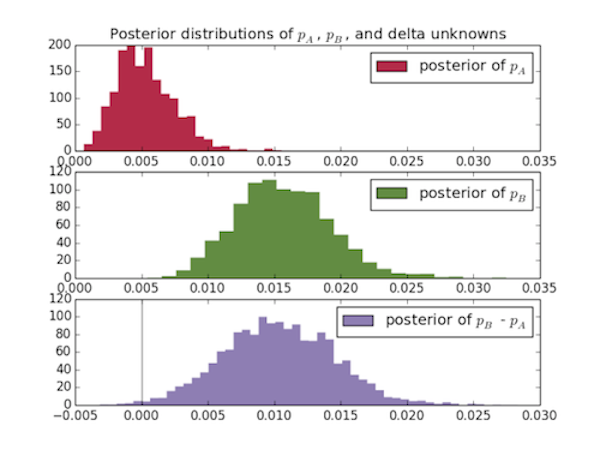
Then I plot the posterior distributions for the three unknowns:

p_A_samples = mcmc.trace("p_A")[:]
p_B_samples = mcmc.trace("p_B")[:]
delta_samples = mcmc.trace("delta")[:]

ax = plt.subplot(311)

plt.xlim(0, .035)
plt.hist(p_A_samples, histtype='stepfilled', bins=25, alpha=0.85,
label="posterior of $p_A$", color="#A60628", normed=True,
edgecolor= "none")
plt.legend(loc="upper right")
plt.title("Posterior distributions of $p_A$, $p_B$, and delta
unknowns")

ax = plt.subplot(312)

plt.xlim(0, .035)
plt.hist(p_B_samples, histtype='stepfilled', bins=25, alpha=0.85,
        label="posterior of $p_B$", color="#467821", normed=True,
        edgecolor = "none")
plt.legend(loc="upper right")

ax = plt.subplot(313)
plt.ylim(0,120)
plt.hist(delta_samples, histtype='stepfilled', bins=50, alpha=0.85,
        label="posterior of $p_B$ - $p_A$", color="#7A68A6",normed=True,
        edgecolor = "none")
plt.legend(loc="upper right")
plt.vlines(0, 0, 120, color="black", alpha = .5)

plt.show()

I can also compute the probability that the true conversion rate of page A, p_A, is better than the true conversion rate of page B, p_A:

print "Probability site A is BETTER than site B: %.3f" %
(delta_samples < 0).mean()
print "Probability site A is WORSE than site B: %.3f" %
(delta_samples > 0).mean()

This should print out:

Probability page A is BETTER than page B: 0.006
Probability page A is WORSE than page B: 0.994

It's very safe to say (as long as our data was collected properly) that page B is better than page A, and these results come very intuitively from looking at the graphs.

The full code can be found on my GitHub.

tags: ab testing matplotlib numpy pymc python